Statistical image processing: segmentation, phenotyping, and normalization
Slide Deck
Overview
This module performs and evaluates intensity normalization on images
from the lung cancer dataset using the mxnorm package.
Load data and libraries.
library(tidyverse)
library(viridis)
library(patchwork)

# load processed lung cancer data
load(url("https://github.com/julia-wrobel/MI_tutorial/raw/main/Data/lung.RDA"))

# for computational reasons, I will perform on a subset of the data with 20 subjects
ids = sample(unique(lung_df$patient_id), 20)
lung_df  = lung_df %>% filter(patient_id %in% ids)
Normalization
We will use the mxnorm package to normalize the lung
data. More examples for working with this package are available in the
package
vignette.
Setting up mx_dataset object
The mxnorm package uses an S3 object-oriented framework
in R to define an mx_dataset which all operations are performed on.
- Use
patient_idas slide identifier - Use
image_idas image identifier - Use the following marker columns:
cd19cd14cd3cd8hladrckdapi
- Use
tissue_categoryas a metadata column
# load the package
# install.packages("mxnorm")
library(mxnorm)

# define the mx_dataset
mx_data = mx_dataset(data = lung_df,
                     slide_id = "patient_id",
                     image_id = "image_id",
                     marker_cols = c("cd19",
                                     "cd3",
                                     "cd14",
                                     "cd8",
                                     "hladr",
                                     "ck",
                                     "dapi"
                                     ),
                     metadata_cols = c("tissue_category",
                                       "phenotype_ck",
                                       "phenotype_cd8",
                                       "phenotype_cd14",
                                       "phenotype_other",
                                       "phenotype_cd19"))


class(mx_data)
## [1] "mx_dataset"
summary(mx_data)
## Call:
## `mx_dataset` object with 20 slide(s), 7 marker column(s), and 6 metadata column(s)
Normalize using mx_normalize()
Here we normalize using the transformation:
log10mean_divide. Then, we calculate Otsu discordance
metrics.
mx_norm = mx_normalize(mx_data,
                       transform = "log10_mean_divide",
                       method = "None")


# Otsu
mx_norm = run_otsu_discordance(mx_norm,
                            table="both",
                            plot_out = FALSE)
Summary table that calculates the metrics from the Bioinformatics paper is printed below:
# calculate metrics for unnormalized and normalized data
summary(mx_norm)
## Call:
## `mx_dataset` object with 20 slide(s), 7 marker column(s), and 6 metadata column(s)
##
## Normalization:
## Data normalized with transformation=`log10_mean_divide` and method=`None`
##
## Anderson-Darling tests:
##       table mean_test_statistic mean_std_test_statistic mean_p_value
##  normalized              81.924                  19.064            0
##         raw             196.099                  53.654            0
##
## Threshold discordance scores:
##       table mean_discordance sd_discordance
##  normalized            0.047          0.051
##         raw            0.103          0.105
Lower values of these metrics indicate better normalization.
Plotting
First, density plots. The code below constructs density plots of normalized and unnormalized CD14 values for 3 subjects.
set.seed(103001)
ids = sample(unique(lung_df$patient_id), 3)
markers = c("cd19", "cd14")

mx_df = mx_norm$data %>%
  mutate(cd14_norm = mx_norm$norm_data$cd14) %>%
  dplyr::select(patient_id, image_id, cd14, cd14_norm) %>%
  pivot_longer(cd14:cd14_norm,
               names_to = "marker",
               values_to = "marker_value") %>%
  filter(patient_id %in% ids)


mx_df %>%
  ggplot() +
  geom_line(stat = "density", aes(marker_value, group = image_id,
                                  color = patient_id),
            alpha=0.5, linetype = 2) +
    geom_density(aes(marker_value, group = patient_id,
                   color = patient_id), size = 1.25) +
  scale_color_viridis(discrete = TRUE) +
  facet_wrap(~marker) +
  #theme(legend.position = "none") +
  xlim(0, 1) +
  labs(x = "")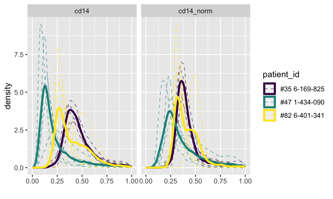
The next set of plots shows Otsu discordance scores. Otsu thresholds were calculated at the slide-level for each marker and compared to a global Otsu threshold for each marker to calculate a discordance score.
Discordance scores are plotted for all 20 subjects and 6 markers, both before and after normalization. The white diamond represents the mean discordance score across all markers for a given method. Given that this is a discordance score, lower values indicate better agreement across slides.
otsu_data = mx_norm$otsu_data %>%
  filter(marker %in% c("cd14", "cd19", "cd8", "cd3", "dapi", "ck")) %>%
  mutate(slide_id = as.numeric(factor(slide_id)),
         norm = factor(table, levels = c("raw", "normalized")))

point_size = 2


mean_vals = otsu_data %>%
  group_by(norm, slide_id) %>%
  summarize(m1 = mean(discordance_score), .groups = "drop")


otsu_data %>%
  ggplot() +
  geom_point(aes(discordance_score, slide_id, color = marker), size = point_size) +
  facet_wrap(~ norm) +
  geom_point(data = mean_vals, aes(m1, slide_id), color = "black", fill = "white",
             shape = 23, size = point_size) +
  labs(x = "discordance score", y = "slide_id")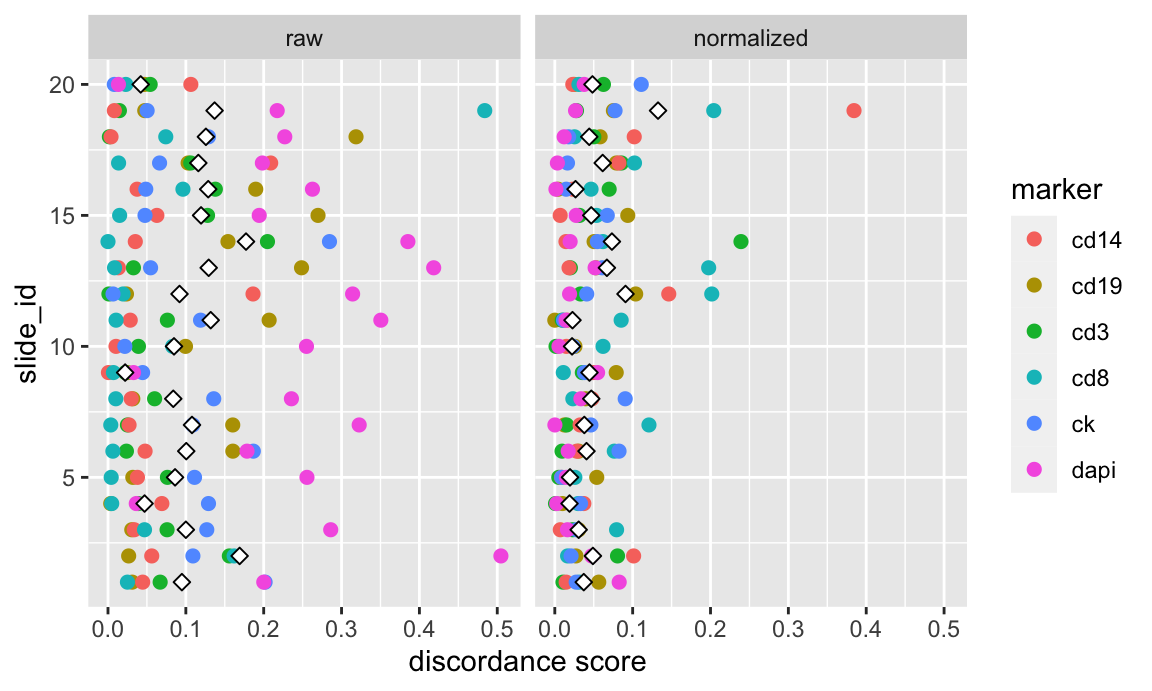
It is also possible to evaluate user-defined normalization using the
mxnorm package. See here
in the package vignette for an example.
References
- textbook chapter, Wrobel and Vandekar
- Challenges and Opportunities in the Statistical Analysis of Multiplex Immunofluorescence Data