VectraPolarisData: experiment-scale multiplex imaging data
Slide Deck
Overview
The VectraPolarisData ExperimentHub package provides two large multiplex immunofluorescence datasets collected using Akoya Biosciences Vectra 3 and Vectra Polaris platforms. Image preprocessing (cell segmentation and phenotyping) was performed using inForm software. Data are provided as objects of class SpatialExperiment.
# load libraries
library(tidyverse)
Install and load data
The data is publicly available on Bioconductor as the package
VectraPolarisData. You can install the package from
Bioconductor here:
if (!requireNamespace("BiocManager", quietly = TRUE)) {
     install.packages("BiocManager")
}

BiocManager::install("VectraPolarisData")
Ovarian cancer data
Load the high grade serous ovarian cancer data. This dataset has been segmented and phenotyped, and has one image per patient.
library(VectraPolarisData)

# load spatial experiment object
oc <- HumanOvarianCancerVP()
Inspect the SpatialExperiment object.
# check object
oc
## class: SpatialExperiment
## dim: 10 1610431
## metadata(1): clinical_data
## assays(3): intensities nucleus_intensities membrane_intensities
## rownames(10): ck_opal_780 ki67_opal_690 ... dapi autofluorescence
## rowData names(0):
## colnames: NULL
## colData names(195): cell_id tissue_category ... phenotype_cd8 sample_id
## reducedDimNames(0):
## mainExpName: NULL
## altExpNames(0):
## spatialCoords names(2) : cell_x_position cell_y_position
## imgData names(0):
The object stores the following marker values for each marker and each cell
intensities: mean marker intensity for entire cellnucleus_intensities: mean marker intensity in the nucleusmembrane_intensities: mean marker intensity in the cell membrane
assayNames(oc)
## [1] "intensities"          "nucleus_intensities"  "membrane_intensities"
Row names provide the names of the markers.
rownames(oc)
##  [1] "ck_opal_780"      "ki67_opal_690"    "cd8_opal_650"     "ier3_opal_620"
##  [5] "p_stat3_opal_570" "cd3_opal_540"     "cd68_opal_520"    "cd19_opal_480"
##  [9] "dapi"             "autofluorescence"
The colData slot contains cell-level covariates like cell phenotype, cell area, and, min, max, and standard deviation of intensity values for each marker.
dim(colData(oc))
## [1] 1610431     195
Many of the variables are summary statistics of marker intensity values. More information on the different variables in this and the lung cancer dataset can be found in the package vignette.
set.seed(12333)
sample(names(colData(oc)), 15)
##  [1] "entire_cell_cd3_opal_540_std_dev"   "nucleus_ki67_opal_690_std_dev"
##  [3] "entire_cell_dapi_dapi_min"          "entire_cell_cd3_opal_540_min"
##  [5] "cytoplasm_cd68_opal_520_total"      "cytoplasm_dapi_dapi_min"
##  [7] "entire_cell_cd8_opal_650_max"       "entire_cell_dapi_dapi_total"
##  [9] "cytoplasm_p_stat3_opal_570_std_dev" "membrane_ier3_opal_620_std_dev"
## [11] "entire_cell_cd3_opal_540_total"     "entire_cell_p_stat3_opal_570_max"
## [13] "nucleus_cd3_opal_540_total"         "membrane_p_stat3_opal_570_max"
## [15] "nucleus_cd68_opal_520_min"
Converting to dataframe
Storing the data as a SpatialExperiment allows for
analysis using tools that are built into the
SpatialExperiment workflow. However, it is often useful to
work with the data as a data.frame object instead.
Code below converts the ovarian cancer dataset from a
SpatialExperiment object to a data.frame. We
perform some data cleaning steps as well.
## Assays slots
assays_slot <- assays(oc)
intensities_df <- assays_slot$intensities
nucleus_intensities_df<- assays_slot$nucleus_intensities
rownames(nucleus_intensities_df) <- paste0("nucleus_", rownames(nucleus_intensities_df))
membrane_intensities_df<- assays_slot$membrane_intensities
rownames(membrane_intensities_df) <- paste0("membrane_", rownames(membrane_intensities_df))

# colData and spatialData
colData_df <- colData(oc)
spatialCoords_df <- spatialCoords(oc)

# clinical data
patient_level_ovarian <- metadata(oc)$clinical_data %>%
  # create binary stage variable
  dplyr::mutate(stage_bin = ifelse(stage %in% c("1", "2"), 0, 1))

# only include samples for whom we have an id in the patient dataset, which is 128- the other 4 are controls
# give Markers shorter names
cell_level_ovarian <- as.data.frame(cbind(colData_df,
                                     spatialCoords_df,
                                     t(intensities_df),
                                     t(nucleus_intensities_df),
                                     t(membrane_intensities_df))
                               ) %>%
  dplyr::rename(cd19 = cd19_opal_480,
                cd68 = cd68_opal_520,
                cd3 = cd3_opal_540,
                cd8 = cd8_opal_650,
                ier3 = ier3_opal_620,
                pstat3 = p_stat3_opal_570,
                ck = ck_opal_780,
                ki67 = ki67_opal_690) %>%
  # define cell type 'immune'
  mutate(immune = ifelse(phenotype_cd19 == "CD19+" | phenotype_cd8 == "CD8+" |
              phenotype_cd3 == "CD3+" | phenotype_cd68 == "CD68+", "immune", "other")) %>%
  dplyr::select(contains("id"), tissue_category, contains("phenotype"),
                contains("position"), ck:dapi, immune) %>%
  # only retain 128 subjects who have clinical data (other 4 are controls)
  dplyr::filter(sample_id %in% patient_level_ovarian$sample_id)


# data frame with clinical characteristics where each row is a different cell
ovarian_df <- full_join(patient_level_ovarian, cell_level_ovarian, by = "sample_id") %>%
  mutate(sample_id = as.numeric(as.factor(sample_id))) %>%
  filter(tissue_category != "Glass") %>%
  dplyr::select(sample_id, cell_id, tissue_category, x = cell_x_position, y = cell_y_position,
                everything()) %>%
  select(-tma, -diagnosis, -grade)

rm(oc, assays_slot, intensities_df, nucleus_intensities_df, membrane_intensities_df, colData_df, spatialCoords_df, patient_level_ovarian, cell_level_ovarian)
The resulting dataframe, ovarian_df, contains
information on marker intensities, cell X and Y position, cell
phenotypes, and patient-level characteristics.
Exploratory analysis
dim(ovarian_df)

head(ovarian_df)

glimpse(ovarian_df)
Below we plot the cells for a single subject. In this dataset there is one image for each subject, and the image comes from a tumor microarray (TMA).
id = sample(ovarian_df$sample_id, 1)

ovarian_df %>%
  filter(sample_id == id) %>%
  ggplot(aes(x, y)) +
  geom_point(aes(color = tissue_category), size = 0.1)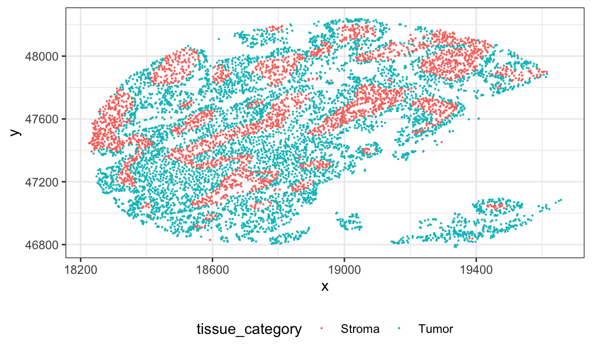
Now we plot the images (below) for multiple subjects. In this dataset, multiple TMA cores (each TMA core is frome a different subject) were placed on the same slide, and then that slide was imaged. X and Y locations in this data correspond to position on the slide for a given patient sample.
ovarian_df %>%
  filter(sample_id < 10) %>%
  ggplot(aes(x, y)) +
  geom_point(aes(color = tissue_category), size = 0.1)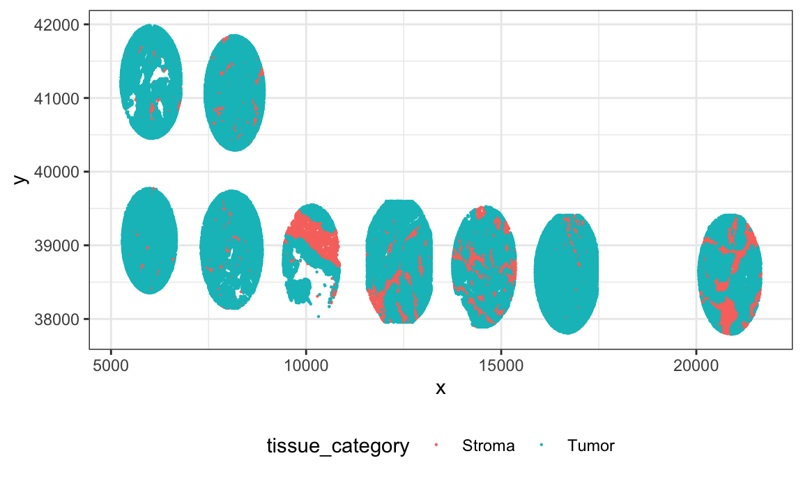
Lung data
Load the non small cell lung carcinoma data and inspect the
SpatialExperiment object. This dataset has 3-4 images per
patient, representing different ROIs from a tissue slice. In this
dataset, each patient was imaged on a separate slide.
# load lung data
lung <- HumanLungCancerV3()
## see ?VectraPolarisData and browseVignettes('VectraPolarisData') for documentation
## loading from cache

# check object
lung
## class: SpatialExperiment
## dim: 8 1604786
## metadata(1): clinical_data
## assays(3): intensities nucleus_intensities membrane_intensities
## rownames(8): cd19_opal_650 cd3_opal_520 ... dapi autofluorescence
## rowData names(0):
## colnames: NULL
## colData names(124): cell_id tissue_category ... phenotype_cd4 sample_id
## reducedDimNames(0):
## mainExpName: NULL
## altExpNames(0):
## spatialCoords names(2) : cell_x_position cell_y_position
## imgData names(0):
Converting to dataframe
Code below converts the lung cancer dataset from a
SpatialExperiment object to a data.frame.
## Assays slots
assays_slot <- assays(lung)
intensities_df <- assays_slot$intensities
nucleus_intensities_df<- assays_slot$nucleus_intensities
rownames(nucleus_intensities_df) <- paste0("nucleus_", rownames(nucleus_intensities_df))
membrane_intensities_df<- assays_slot$membrane_intensities
rownames(membrane_intensities_df) <- paste0("membrane_", rownames(membrane_intensities_df))

# colData and spatialData
colData_df <- colData(lung)
spatialCoords_df <- spatialCoords(lung)

# clinical data
patient_level_lung <- metadata(lung)$clinical_data

cell_level_lung <- as_tibble(cbind(colData_df,
                                     spatialCoords_df,
                                     t(intensities_df),
                                     t(nucleus_intensities_df),
                                     t(membrane_intensities_df))
                               )   %>%
  dplyr::rename(cd19 = cd19_opal_650,
                cd3 = cd3_opal_520,
                cd14 = cd14_opal_540,
                cd8 = cd8_opal_620,
                hladr = hladr_opal_690,
                ck = ck_opal_570) %>%
  dplyr::select(cell_id:slide_id, sample_id:dapi,
                entire_cell_axis_ratio:entire_cell_area_square_microns, contains("phenotype"))


# data frame with clinical characteristics where each row is a different cell
lung_df <- full_join(patient_level_lung, cell_level_lung, by = "slide_id") %>%
  #mutate(slide_id = as.numeric(as.factor(slide_id))) %>%
  dplyr::select(image_id = sample_id, patient_id = slide_id,
                cell_id, x = cell_x_position, y = cell_y_position,
                everything())

rm(lung, assays_slot, intensities_df, nucleus_intensities_df, membrane_intensities_df, colData_df, spatialCoords_df, patient_level_lung,
   cell_level_lung)
The resulting dataframe, lung_df, contains information
on marker intensities, cell X and Y position, cell phenotypes, and
patient-level characteristics.
Exploratory analysis
Below shows images from a single subject. Each image represents a different ROI from the same tissue slice from a single subject. There are 3-6 ROIs for each subject.
id = sample(lung_df$patient_id, 1)

lung_df %>%
  filter(patient_id == id) %>%
  ggplot(aes(x, y)) +
  geom_point(aes(color = tissue_category), size = 0.1) +
  facet_wrap(~image_id)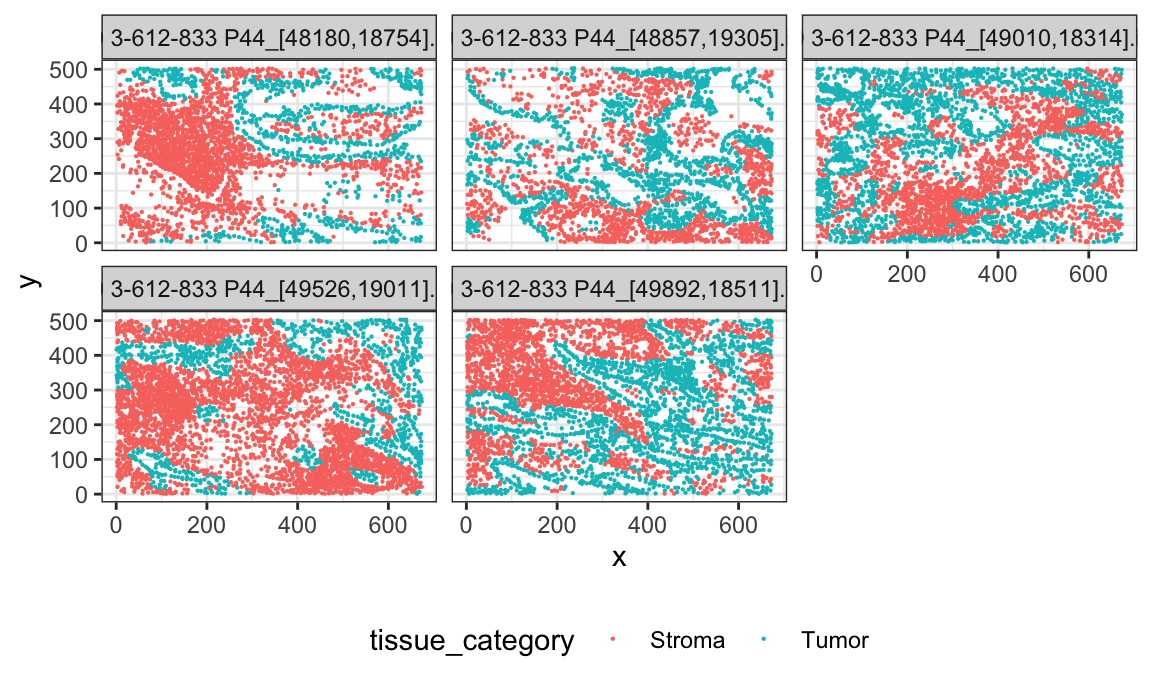
Data saving
Processed data are saved as .rda objects and can also be
downloaded directly from the short course website. For the rest of the
workshop we will be working with this processed data.
# save data sets
save(ovarian_df, file = here::here("Data", "ovarian.RDA"))
save(lung_df, file = here::here("Data", "lung.RDA"))

# load processed ovarian data
load(url("https://github.com/julia-wrobel/MI_tutorial/raw/main/Data/ovarian.RDA"))

# load processed lung data
load(url("https://github.com/julia-wrobel/MI_tutorial/raw/main/Data/lung.RDA"))
References
Original citations for the two datasets in the
VectraPolarisData package, and the package vignette which
includes a data dicitonary:
- Vignette for VectraPolarisData
- Paper for ovarian cancer data
- Paper for non-small cell lung carcinoma data
More resources for SpatialExperiment: