Introduction to multiplex single-cell imaging data
Slide Deck
Overview
In this module I briefly discuss loading and visualizing raw TIFF data. The rest of the workshop will focus on data in tabular form post segmentation.
Lung cancer data
The following image is a single ROI from a tissue slice from a patient with non small cell lung carcinoma.Cell and tissue segmentation and cell phenotyping were performed using inForm software. For each image, there are multiple Tiff files output by inForm:
lung_component_data.tif: the multichannel file we are most interested inlung_binary_seg_maps.tif: 3 channel file with binary segmentation mapslung.tif: A composite image in RGB format.
You can download these files from the Data tab and store them in a local directory.
#BiocManager::install("EBImage")

# load relevant libraries
library(tidyverse)
library(tiff)
library(EBImage)


# define your specific file path
my_path = "./Data/"

# define file for different .tif files
component = paste0(my_path, "lung_component_data.tif")
binseg = paste0(my_path, "lung_binary_seg_maps.tif")
composite_tif = paste0(my_path, "lung.tif")
Component file
The component.tif file contains the multichannel tiff,
which is a stack 0f individual images (one for each marker). Below I
define a function to read the component file and extract metadata.
# this function is from phenoptr package on GitHub
# extracts metadata specific to Vectra3/VectraPolaris images
read_components <- function(path) {
  stopifnot(file.exists(path), endsWith(path, 'component_data.tif'))

  # The readTIFF documentation for `as.is`` is misleading.
  # To read actual float values for components, we want `as.is=FALSE`.
  tif = tiff::readTIFF(path, all=TRUE, info=TRUE)

  # Get the image descriptions and figure out which ones are components
  infos = purrr::map_chr(tif, ~attr(., 'description'))
  images = grepl('FullResolution', infos)

  # Get the component names
  names = stringr::str_match(infos[images], '<Name>(.*)</Name>')[, 2]

  purrr::set_names(tif[images], names)
}

image_stack = read_components(component)
The image_stack object is now a list, where each list
element is a different marker
map(image_stack, dim)
## $`CD19 (Opal 650)`
## [1] 1008 1348
##
## $`CD3 (Opal 520)`
## [1] 1008 1348
##
## $`CD14 (Opal 540)`
## [1] 1008 1348
##
## $`CD8 (Opal 620)`
## [1] 1008 1348
##
## $`HLADR (Opal 690)`
## [1] 1008 1348
##
## $`CK (Opal 570)`
## [1] 1008 1348
##
## $`DAPI (DAPI)`
## [1] 1008 1348
##
## $Autofluorescence
## [1] 1008 1348
I can use the display() function from the
EBImage package to plot an individual channel. Below the
DAPI (nucleus) channel is plotted.
dapi_channel = t(image_stack$"DAPI (DAPI)")
EBImage::display(dapi_channel, method = "raster")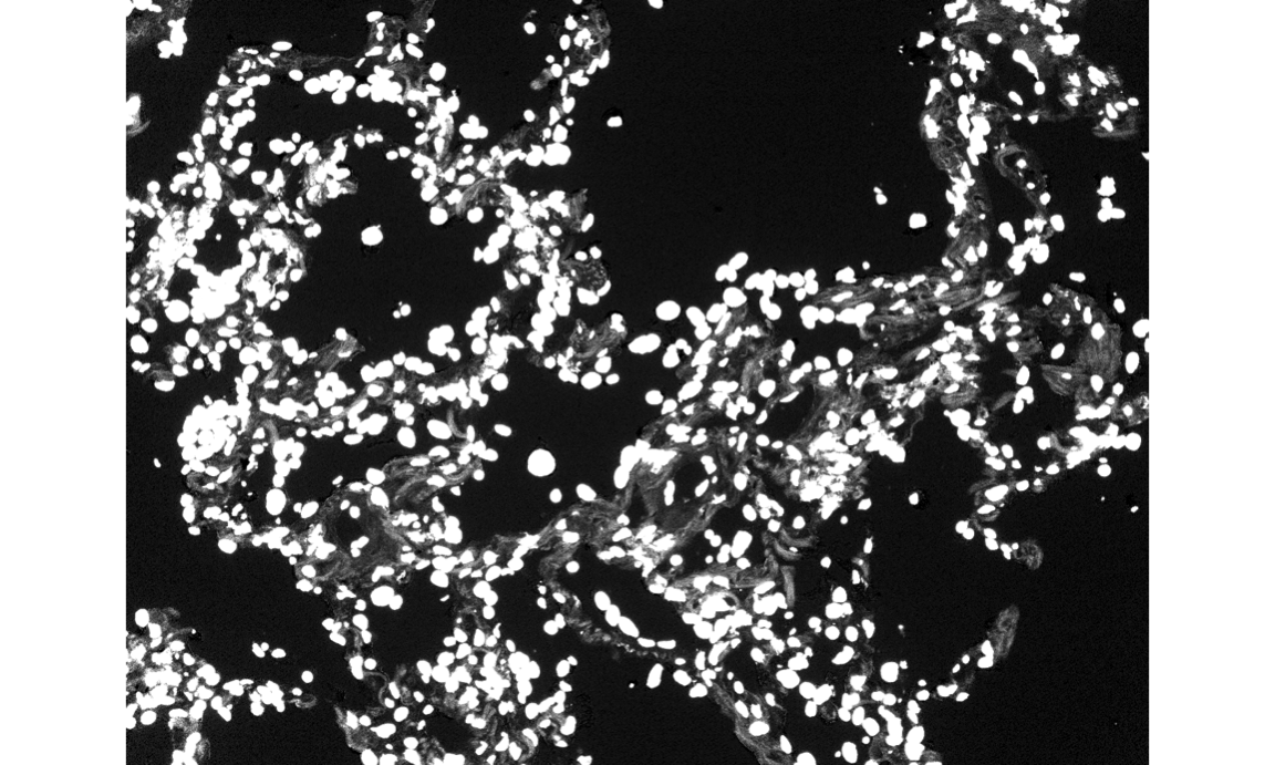
# plot the image in a specified color
dapi = rgbImage(blue=.1*dapi_channel, red = .02 * dapi_channel)
display(dapi, method = "raster")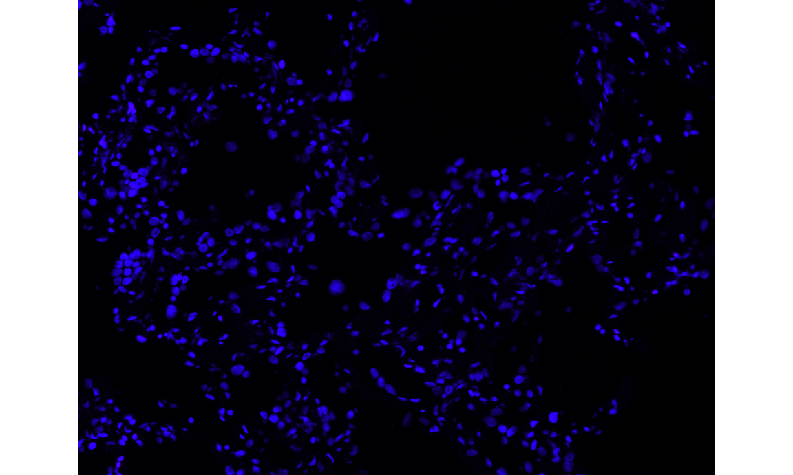
Segmentation files
This data was collected on a Vectra 3 instrument and segmented using inForm tissue analysis software from Akoya Biosciences. This is proprietary image analysis software that can perform cell and tissue segmentation and cell phenotyping. The segmentation below were performed by that software.
# source phenoptr code for loading file and metadata, based on tiff::readTIFF.
source("https://raw.githubusercontent.com/akoyabio/phenoptr/main/R/read_maps.R")

segmentations = read_maps(binseg)
names(segmentations)
## [1] "Nucleus"  "Membrane" "Tissue"
Nucleus segmentation
nucleus = segmentations[['Nucleus']]
plot(as.raster(nucleus, max = max(nucleus)))
Tissue segmentation
tissue = segmentations[['Tissue']]

plot(as.raster(tissue, max = max(tissue)))
Composite file
# source phenoptr code for loading file and metadata, based on tiff::readTIFF.
source("https://raw.githubusercontent.com/akoyabio/phenoptr/main/R/read_composites.R")

composite = read_composites(composite_tif)
composite = as.raster(composite[[1]])
plot(composite)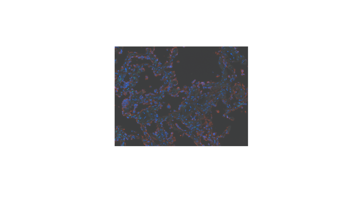
References
Below are original citations for the two example datasets I will be working with in this tutorial.
Resources from Akoya Biosciences on working with this data
Below are some references that review this rapidly growing area.