Learning Shiny with NBA data
Shiny is R Studio’s framework for building interactive plots and web
applications in R. By the end of this tutorial you should
have some basic understanding of how Shiny works, and will make and
deploy a Shiny app using NBA shots data. Thanks to Todd Schneider’s ballR
app inspiration.
Getting started
Before we begin, make sure you have the shiny,
plotly, tidyverse, and rsconnect
packages installed. I have created a template for our app and completed version, please
download and unzip these folders as well.
install.packages(c("shiny", "plotly", "tidyverse", "rsconnect"))Run an example of a simple shiny app to ensure the package is installed properly.
library(shiny)
runExample("01_hello")
A slider bar the allows you to change the number bins in the histogram shown.
Shiny basics
Each Shiny app has a ui and a server file,
both of which we have to define. The ui defines a webpage
that the user interacts with, it controls layout and appearance. The
server file is a set of instructions your computer needs to
build the app. R code is executed in the background, and
output depends on the user input and this R code.
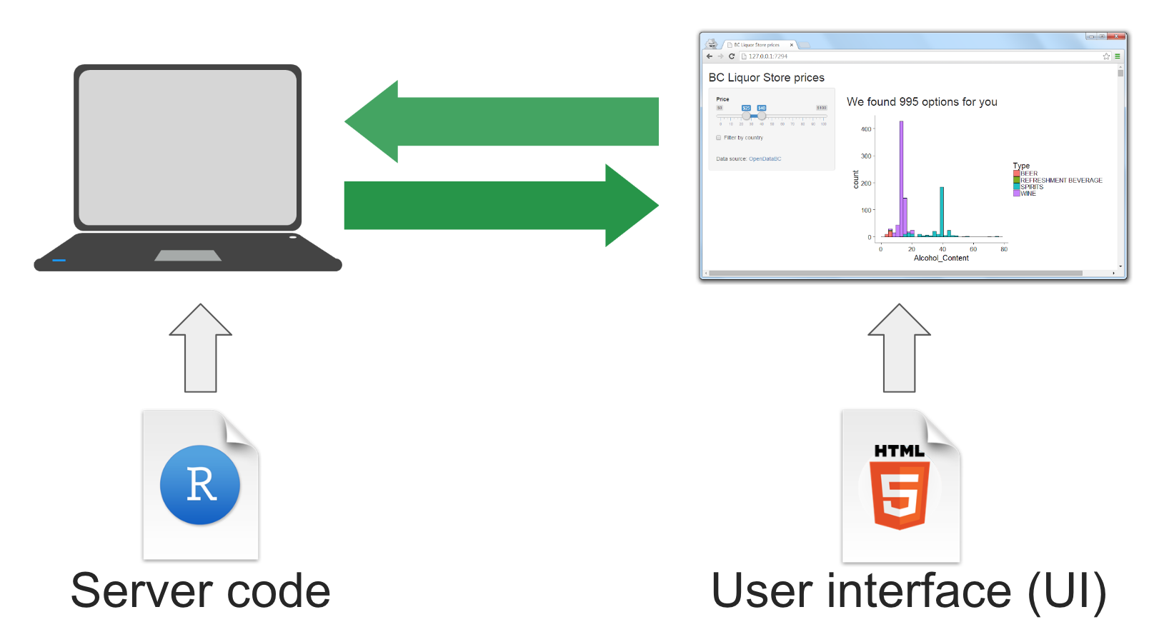
image from https://deanattali.com/blog/building-shiny-apps-tutorial/
The shiny framework
All Shiny apps follow the same overall structure.
fluidPage() controls the page layout for the UI. The
server is a function with arguments input and
output.
library(shiny)
ui <- fluidPage()
server <- function(input, output) {}
shinyApp(ui = ui, server = server)
This template itself is a minimal Shiny app, try running the code.
Copy this template into a new file called app.R, and save
it in a new folder. After saving the file, you should see a Run
App button at the top, indicating R Studio has recognized the file
as a Shiny app.
![]()
There are two ways to create Shiny apps:
- Put both the UI and the server code into single file called
app.R, ideal for simple apps. If you are using a single file, the file must be calledapp.Rfor the app to run. - Create separate
ui.Randserver.Rfiles, ideal for more complicated apps. These must be namedui.Randserver.R. Our NBA app uses this approach.
You can initialize a Shiny app using either approach right from R Studio:
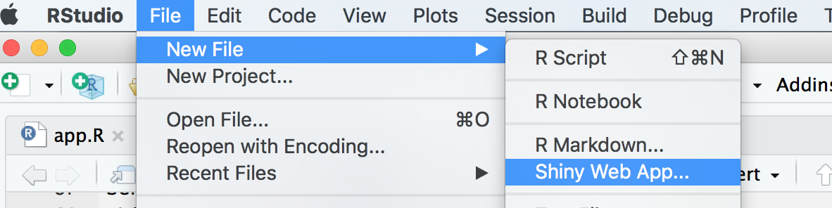
Select Shiny Web App… and the following will pop up:
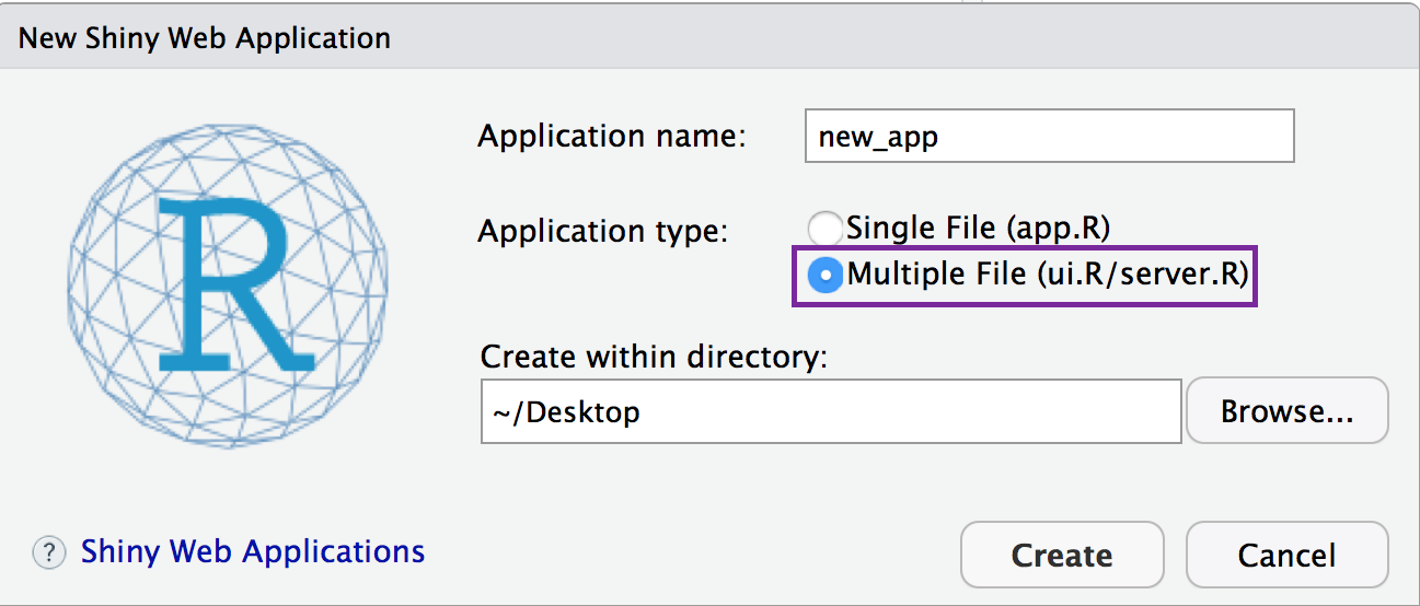
Select Multiple File to generate an app with
separate ui.R and server.R files. The app
initialized above will be stored in a folder called “new_app” on the
Desktop. To run the app you can do either of the following:
- Open the
server.Rorui.Rfile and click the Run App button. - Enter
shiny::runApp("~/Desktop/new_app/")in your R console
The input and output arguments to the server function are actually lists of objects defined in the UI. These input options, output options, and server side code called render statements are the main components of most Shiny apps, and are defined below.
Input options
Input options (usually) go in the ui.R file. Input is
defined through input functions called widgets.
These are text elements a user can interact with, like scroll bars or
buttons. Three widget options and the code used to generate them are
shown below.
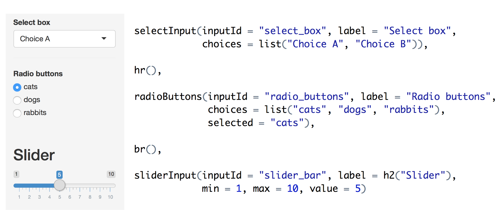
All input functions have inputId and label
as the first two arguments. The inputId is a string that
the server side will use to access the value of the user input. For
example, if inputId = "slider_widget" then on the server
side you would use input$slider_widget to use its
value.label is the title for the widget that will show up
in the UI.
The hr(), br(), and h2() in
the example code above are wrappers for the html tags
<hr> <br>, and
<h2>. There are a bunch of awesome html
wrapper functions to help you customize your user interface.
Output options
Output options (also usually) go in the ui.R file. They
define things like plots and tables and instruct Shiny where in the UI
to place these items. Examples include plotOutput(),
textOutput(), tableOutput().
Debugging tip: Make sure you have a comma between
each input call and output call! Commas are needed between elements for
the UI but not for the server, which operates more like regular
R code.
render* statements
Render statements go in the server.R file. They take
user input from the widgets and build reactive output to display in the
UI. Examples including renderTable() to make tables,
renderText() for text, and renderPlot() for
certain plots.
Input, output, and render statements are the simplest examples of the reactive programming paradigm that Shiny uses. We will cover reactivity in more detail later.
NBA Shots Data
Download and unzip the shiny_nba folder provided. Notice what’s in the folder:
- an R project called
shiny_nba.Rproj - the
nba_shots.RDatadata on shots taken by LeBron James, Kevin Durant, Russell Westbrook, Stephen Curry, and Carmelo Anthony - a
helper.Rfile with extraRcode our app uses - a
ui.Rfile - a
server.Rfile
R project
Double click the shiny_nba.Rproj
to open up R Studio. This automatically sets your working directory to
the shiny_nba folder, which makes it easier to load the
data and source the helper functions. This is one of many reasons I
always use R projects as part of my workflow.
The data
The nba_shots data contains 81,383 basketball shots
taken by five star NBA players.
library(tidyverse)
load("nba_shots.RData")

nba_shots %>%
  group_by(player_name) %>%
  summarize(n())
## # A tibble: 5 × 2
##   player_name       `n()`
##   <fct>             <int>
## 1 LeBron James      22381
## 2 Kevin Durant      14476
## 3 Russell Westbrook 13778
## 4 Stephen Curry     10508
## 5 Carmelo Anthony   20240
The data has 19 variables, including information on shot distance, accuracy, season, and location on the court.
Helper file
The helper.R code is adapted from Todd Schneider’s ballR
app. While the code looks complicated, it is just used to draw the
lines of a basketball court. The empty basketball court (below) is a
ggplot object you can put other ggplot layers on top of.
source("helpers.R")

gg_court = make_court()
gg_court![]()
This code was stored in a separate file in order to make the code
within the Shiny app more readable and because this part of the code
does not change with user input. However, it doesn’t have to be included
as a separate file - all of the code could be placed within the
server.R file instead. Where to put static code like this
is a choice to be made when building a Shiny app.
Court plot
Next let’s add a plot. We are going to plot the locations of the attempted shots made by the selected NBA star in a given season, like LeBron James in his rookie 2003-2004 season (below).
player_data = filter(nba_shots, player_name == "LeBron James", season == "2003-04")

gg_court + geom_point(data = player_data, alpha = 0.75, size = 2.5,
                          aes(loc_x, loc_y, color = shot_made_flag)) +
  scale_color_manual("", values = c(made = "blue", missed = "orange"))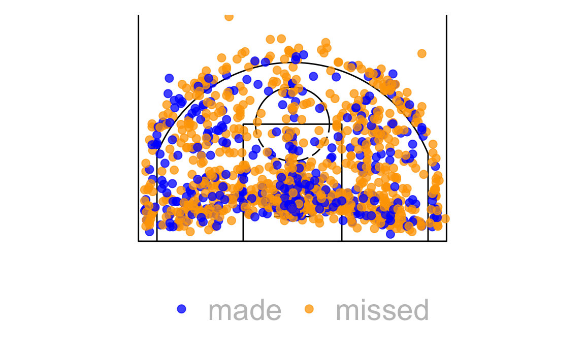
Plotly
Some of the plots for our app use Plotly, which is a framework for
creating interative graphics that has a variety of implementations,
including the plotly library in R. Plotly has
some nice benefits:
- High quality plots produced with a few lines of code
- Since (unlike in Shiny) its interactivity does not require running a server, plots can be placed in R Markdown documents that are hosted on GitHub (like this tutorial)!
- Compatible with Shiny framework, making additional interactivity possible
We can make Plotly box plot of shooting distances for our NBA players with just two lines of code. Notice that you can hover, zoom, unclick players, and download the image.
library(plotly)

plot_ly(data = nba_shots, y = ~shot_distance, color = ~player_name, type = "box") %>%
layout(legend = list(x = 0.2, y = 1.0))Note: There is also a Plotly wrapper,
ggplotly, for ggplot2 objects. The code below makes a box
plot using ggplot() then translates it to Plotly. This can
be useful for making quick plots if you want Plotly functionality but
you’re more used to ggplot2 syntax. From my experience the
plot_ly() function works better than the
ggplotly() function, so I would usually recommend using the
plot_ly function or just sticking with
ggplot() if you don’t need the extra interactivity. I do
use ggplotly() to quickly identify outliers when doing
exploratory analysis on a new dataset.
nba_boxplot = nba_shots %>%
  filter(shot_made_flag == "made") %>%
  ggplot(aes(player_name, shot_distance, fill = player_name)) + geom_boxplot() +
  theme(legend.position = "none")

ggplotly(nba_boxplot)
This time I also filtered out missed shots because I was curious how many of the shots taken really far away were actually made. Steph Curry makes the most far shots on average (turns out this is one of his trademarks, which I didn’t know being a basketball neophyte) – but the outliers belong to LeBron!
In 2007 LeBron made an 82 foot shot in a game against the Celtics, as the buzzer indicated the end of the 3rd quarter.
NBA Shots App
I refer back to what’s in the shiny_nba folder. The
ui.R and server.R files define the actual
Shiny app.
- a
ui.Rfile - a
server.Rfile - an R project called
shiny_nba.Rproj - the
nba_shots.RDatadata - a
helper.Rfile
Run the app by opening the shiny_nba.Rproj then typing
runApp() into your console or opening the ui.R
or server.R file and clicking the Run App button. You
should see a simple app with only the title “NBA Shot Attempts”, because
code for widgets and plots has been commented out.
Sidebar layout
The app has a gray box on the left side, called the side bar, which
is where we will place widgets. The white space on the right side is
called the main panel, and this is where we place plots. This design is
called sidebarLayout(). Many more
flexible layouts are possible as well, but we won’t cover them here.
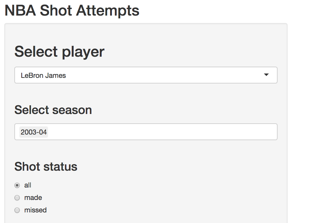
Uncomment the following line in the ui.R to add our first
widget, a drop down menu that allows the user to select a basketball
player.
## uncomment in ui.R
selectInput("player_choice", label = h3("Select player"),
            choices = players, selected = "LeBron James") #, # uncomment comma to add another widget
We also want a widget that allows the user to select a particular
season of play for a given player. But that requires the
possible choice of seasons to depend on the player_choice
input! By adding a uiOutput() statement in
ui.R and a renderUI() statement in
server.R we allows the UI options to adapt to user input.
Uncomment the following code in your app.
## uncomment in ui.R
uiOutput("season_choice") #,

## uncomment in server.R
output$season_choice <- renderUI({
  seasons = nba_shots %>% filter(player_name == input$player_choice) %>%
    distinct(season) %>% pull()

  selectizeInput("season_choice", label = "Select season", choices = seasons,
                selected = seasons[1], multiple = TRUE)
  })
Getting an error that looks like this?
ERROR: Error sourcing /Users/juliawrobel/Downloads/shiny_nba/ui.R
Make sure to uncomment the , between input calls in the
ui.R file.
Last we’ll add a radio button widget that allows the user to
filter out made or missed shots:
## uncomment in ui.R
radioButtons("shots_made", label = h3("Shot status"), choices = list("all", "made", "missed"))
You should now have the following widgets in your sidebar:
Exercise: add another widget to your UI.
Court plot
Let’s add the plot that shows the spatial distribution of shots on
the court. We need a plotOutput statement in the
ui.R file to tell Shiny where the plot should appear in the
layout of the app, and a renderPlot statement in the
server.R file that constructs the plot.
## uncomment in ui.R
plotOutput("court_shots") #, uncomment comma when adding next plot

## uncomment in server.R
  output$court_shots <- renderPlot({
    # subset data by selected player and season(s)
    player_data = filter(nba_shots, player_name == input$player_choice,
                         season %in% input$season_choice)

    # create plot
    gg_court + geom_point(data = player_data, alpha = 0.75, size = 2.5,
                          aes(loc_x, loc_y, color = shot_made_flag, shape = season)) +
      scale_color_manual("", values = c(made = "blue", missed = "orange"))
  })
Debugging tip: if the non-Shiny version of your plot isn’t working, your Shiny version won’t either! Make sure to test your code before placing it in the Shiny framework.
All of the server code that changes based on user input goes within
the renderPlot statement. We allow the plot to change based
on choices of player or season, which are stored in
input$player_choice and
input$season_choice.
Exercise: try editing the app so that the court shots plot also changes based on the radio button input.
Plotly and Shiny
To add Plotly plots to Shiny apps you need to use the functions
plotlyOutput() and renderPlotly() rather than
plotOutput() and renderPlot(). Add the Plotly
box plot of shooting distances to the shiny_nba app by
uncommenting the code below. We allow the user to filter on whether
shots were made or missed by accessing the input$shots_made
UI input from the radioButtons widget.
## uncomment in ui.R
plotlyOutput("shot_distances")

## uncomment in server.R
output$shot_distances <- renderPlotly({
  nba_shots %>%
    filter(if(input$shots_made != 'all')  (shot_made_flag == input$shots_made) else TRUE) %>%
    plot_ly(y = ~shot_distance, color = ~player_name, type = "box") %>%
    layout(showlegend = FALSE)
  })
Make sure to uncomment the , between output calls in the
ui.R file. No commmas are needed between code chunks in the
server file.
The Plotly Shiny gallery contains many more examples of what’s possible when using Plotly and Shiny together.
Getting fancier
Now you have a cool Shiny app! I’ve included an expanded version of
the app shiny_nba app to show off more stuff Shiny can do. Download it
here, then open the
shiny_nba_complete.Rproj and run the app. The app has a few
updates:
- Reactive expressions in the
server.Rfor more efficient code - Tabbed layout, with one plot on each tab
- New plots on the third and fourth tabs
- Mouse-driven coupled events in the fourth tab
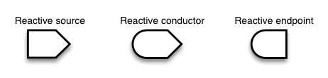
Reactivity
Shiny uses reactive programming, which is what allows output to update based on user input. There are three types of reactive objects in Shiny’s reactive programming paradigm: reactive sources, reactive conducters, and reactive endpoints.
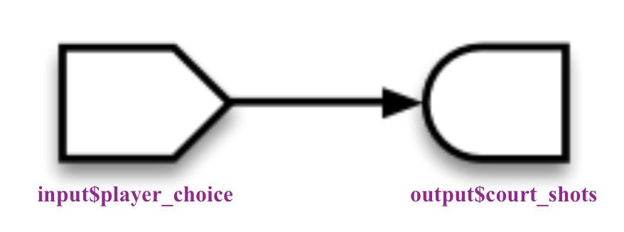
In what we have done so far, input$ statements are the
reactive sources and output$ statements are the reactive
endpoints. We haven’t used any reactive conducters. From our simple
shiny_nba app:
However, sometimes Shiny apps require slow computation, and if one
source has multiple endpoints then these computations will need to be
done several times. Reactive conducters can speed this up. Reactive
expressions are an implementation of reactive conducters that take
an input$ value, do some operation, and cache the
results. The code our_expression = reactive({}) creates a
reactive expression called our_expression. Since reactive
expressions are actually functions, we call the reactive expression
using parenthesis: our_expression().
The fancier shiny_nba_complete app uses a reactive
expression to store a data set that has been filtered on the current
value of input$player_name. In the code below, from
server.R of this app, a dataframe called
player_data is defined using a reactive expression, then
accessed by the reactive endpoint output$court_shots by
calling player_data().
# subset data by selected player using reactive expression
player_data = reactive({
filter(nba_shots, player_name == input$player_choice)
})
# create court_shots plot
output$court_shots <- renderPlot({
gg_court + geom_point(data = filter(player_data(), season %in% input$season_choice),
alpha = 0.75, size = 2.5,
aes(loc_x, loc_y, color = shot_made_flag, shape = season)) +
scale_color_manual("", values = c(made = "blue", missed = "orange"))
})
# create court_position plot
output$court_position <- renderPlot({
# subset data by selected player and season(s)
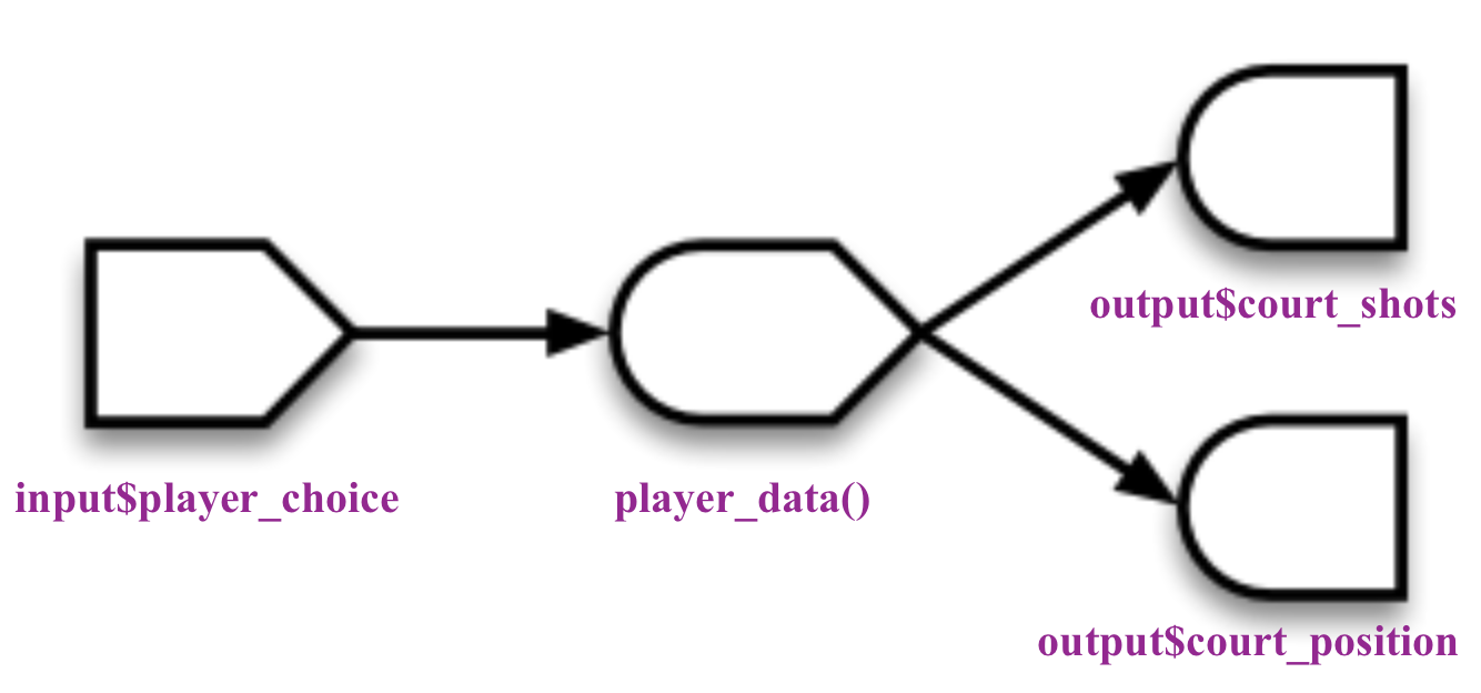
nba_subset = player_data() %>%Since both output$court_shots and
output$court_position use this data, we save ourselves from
doing the computation twice. The reactive diagram for this is:
Coupled events
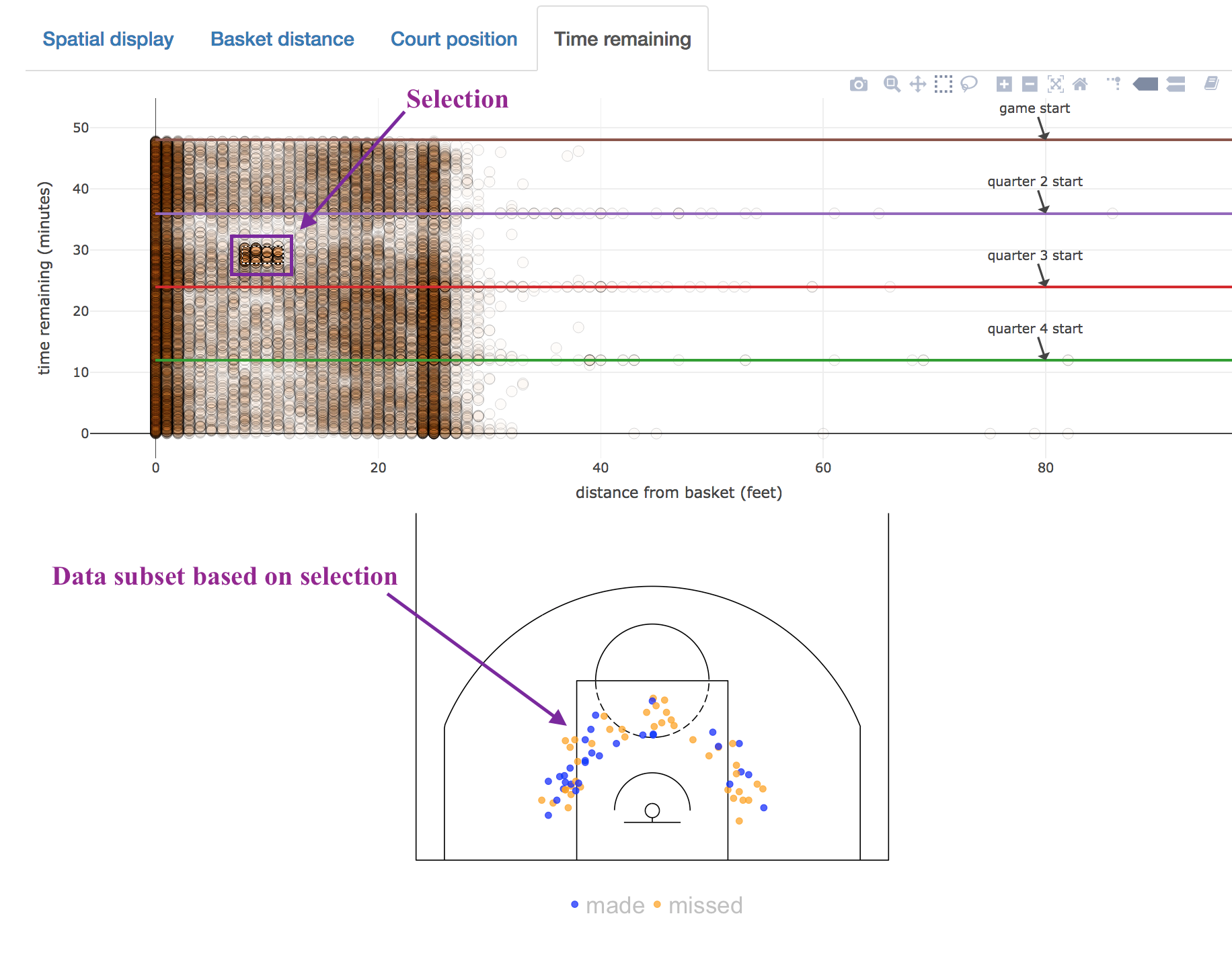
When using Plotly and Shiny together you can use coupled mouse events to create new user-driven plots. Coupled events allow you (for example) to click or select points on a plot and have information based on those clicks or selections show up in another plot. The “Time remaining” tab of the complete app uses coupled events - in the top plot the user can select data points, and the subset of shots that corresponds to the user selection will show up on the plot below.
All code needed to add coupled events to a set of plots goes in the
server.R file. For our coupled event, the first plot is
made using Plotly. The boxed parts of the code below are needed to turn
on mouse event coupling for this plot. In the app, the code for this
plot is much longer, but the rest of the code is just for aesthetics and
doesn’t have anything to do with coupling.
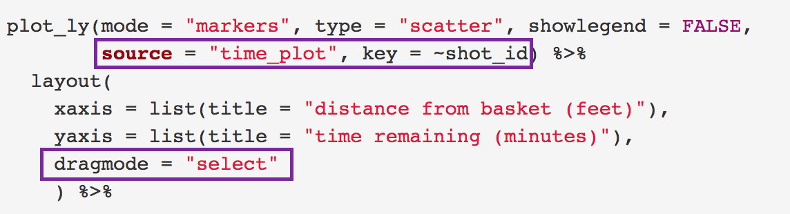
The source = "time_plot" gives your coupled event an id
(which is useful if you want multiple plots to have coupling), and
key = ~shot_id identifies a variable in the dataset that
can you used to access the mouse event data.
The second plot is made using ggplot2, but only data that the user selects on the plot above will show up in this plot.

We access selected data using "plotly_selected". We then
subset the nba_shots data based on the user selection.
To access hover or click data use "plotly_hover" or
"plotly_click", respectively.
Deploying your app
We’ve already run our app locally, but hosting it publicly can be
more tricky. You can’t just host it on GitHub like you would an R
Markdown or blogdown website because R needs to be
running in the background. However, you can publicly host shiny apps at
Shinyapps.io.
The rsconnect package deploys Shiny apps to
shinyapps.io. Load this package and create your own account at shinyapps.io. Once you have created
a shinyapps.io account and configured the rsconnect package
to your account (follow these
instructions, you only have to do it once) you are ready to host
your app. All you have to do is navigate to the folder where your app is
held (so easy if you’re using an R Project!) and run to following
code:
library(rsconnect)
deployApp()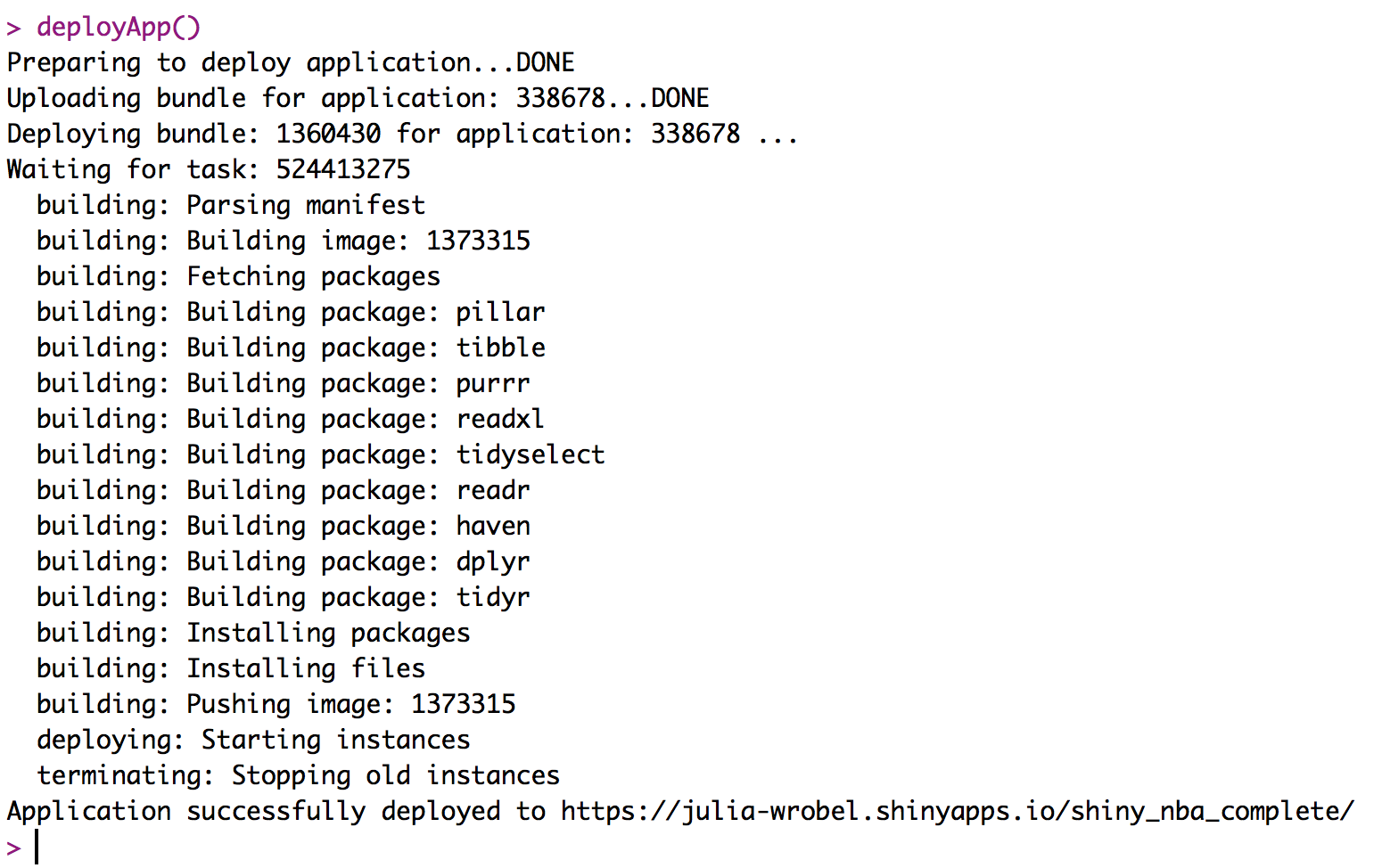
Congrats, you have a published your Shiny app! Mine is hosted here.
A few other things about deployment:
- You can make changes to your app then run
deployApp()again. It should be faster after the first time - Unless you have a special, non-free account you will only be able to host one public Shiny app at a time
- I’ve had trouble deploying Shiny apps when datasets are not in the
same folder as the
ui.Randserver.Rfiles. This is why I put thenba_shots.RDatain the same folder as these other files